Hierarchical Clustering

Hierarchical clustering is a type of unsupervised learning technique used in machine learning for grouping similar objects together. It is based on the idea of creating a hierarchy of clusters where each node in the hierarchy represents a cluster of similar objects. In this technique, the similarity between two objects is measured using a distance metric, and objects that are close to each other are grouped together in a cluster.

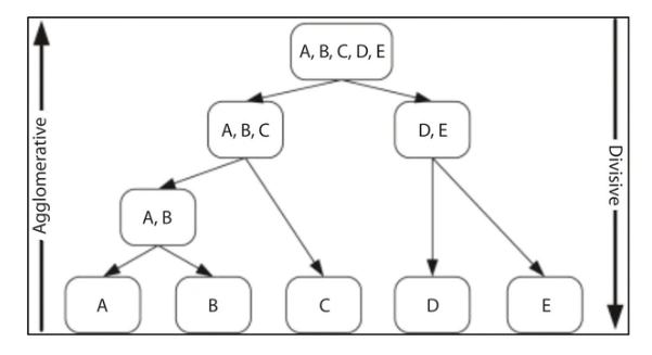
Hierarchical clustering can be of two types: agglomerative and divisive.

Agglomerative clustering is a hierarchical clustering technique used to group data points into clusters based on their similarities. The technique works by starting with each data point as a separate cluster and then iteratively merging the two most similar clusters into a single cluster until a single cluster containing all the data points is formed.

The similarity between clusters is measured using a distance metric such as Euclidean distance or cosine similarity. Initially, each data point is considered as a separate cluster, and the distance between each pair of clusters is calculated using the chosen distance metric. The two closest clusters are then merged, and the distance between the newly formed cluster and the remaining clusters is recalculated. This process continues until all the data points are in a single cluster.

Agglomerative clustering can be visualized using a dendrogram, which is a tree-like diagram that shows the hierarchical relationship between clusters. At the bottom of the dendrogram, each data point is shown as a separate leaf node. As we move up the dendrogram, clusters are formed by merging two or more nodes. The height of each branch in the dendrogram represents the distance between the merged clusters.

Advantages of Agglomerative Clustering

1. Flexibility: Agglomerative clustering is a hierarchical clustering technique, which means it can be used to examine the data at different levels of granularity. This allows for a flexible exploration of the data, from individual data points to larger clusters.
2. Visualization: Agglomerative clustering produces a dendrogram, which is a tree-like diagram that shows the hierarchical relationship between clusters. This dendrogram can be used to visualize the structure of the data and identify any underlying patterns or relationships.
3. Interpretability: Agglomerative clustering produces a set of nested clusters, which can be interpreted as a hierarchy of clusters. This can make the clustering results more interpretable and easier to understand.
4. Handles complex data: Agglomerative clustering can handle large and complex datasets, as it does not make any assumptions about the shape or size of the clusters. This makes it suitable for a wide range of applications, including image segmentation, text clustering, and bioinformatics.
5. No prior knowledge required: Agglomerative clustering does not require any prior knowledge about the number of clusters or their locations. It can automatically determine the optimal number of clusters based on the similarity between the data points.
6. Robustness: Agglomerative clustering is robust to noise and outliers, as it merges similar clusters based on their pairwise distances. This can help to reduce the impact of noisy or irrelevant data on the clustering results.

Disadvantages of Agglomerative Clustering

1. Computational complexity: The computational complexity of agglomerative clustering can be high, especially for large datasets. The time complexity of the algorithm is O(n^3), where n is the number of data points, which makes it impractical for very large datasets.
2. Sensitivity to noise: Agglomerative clustering can be sensitive to noise and outliers in the data. Outliers can lead to the formation of separate clusters, which can affect the overall clustering results.
3. Sensitivity to the choice of distance metric: The quality of the clustering results can be sensitive to the choice of distance metric used to calculate the similarity between the data points. Different distance metrics can lead to different clustering results.
4. Sensitivity to the choice of linkage criteria: The choice of linkage criteria used to merge the clusters can also affect the quality of the clustering results. Different linkage criteria can lead to different cluster structures and sizes.
5. Lack of scalability: Agglomerative clustering is not scalable to high-dimensional data. The curse of dimensionality can cause the distance between data points to become increasingly similar, making it difficult to distinguish between them.

---

Divisive Clustering

Divisive clustering, also known as top-down clustering, is a hierarchical clustering technique that works by starting with all the data points in a single cluster and then recursively dividing the cluster into smaller and smaller subclusters until each data point is in its own cluster. This technique is the opposite of agglomerative clustering, which starts with each data point as a separate cluster and then merges them together.

Divisive clustering works by iteratively splitting the data into subclusters based on some criterion until a stopping condition is met. The criterion can be based on different factors, such as the variance of the data or the similarity between the data points. The process continues until each data point is in its own cluster or until a predefined number of clusters is reached.

Example

A suitable example of divisive clustering is clustering customers based on their purchase history. Suppose we have a dataset of customers and their purchase history, including the type of products they buy, the frequency of their purchases, and the amount they spend. We want to group the customers into clusters based on their purchasing behavior.

To perform divisive clustering, we could start by considering all the customers as a single cluster. We could then recursively split the cluster into smaller subclusters based on some criterion, such as the amount they spend or the types of products they buy.

For example, we could first split the customers into two subclusters based on their spending behavior, one group that spends a lot and another group that spends less. We could then further divide the high-spending group into subgroups based on the types of products they buy, such as electronics, fashion, or home goods. Similarly, we could divide the low-spending group into subgroups based on their purchase frequency or other criteria.

The process continues until each data point is in its own cluster or until a predefined number of clusters is reached. The final result would be a hierarchical tree structure, called a dendrogram, that shows the clusters at different levels of granularity.

---

Dendrogram

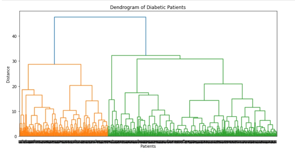
A dendrogram is a tree-like diagram that shows the hierarchical relationships between objects or groups of objects. In the context of diabetic patients, a dendrogram can be used to group patients based on their clinical features, such as age, gender, blood glucose level, and so on. The dendrogram can be helpful in identifying patterns and subgroups of patients that may have different disease outcomes or treatment responses.

The dendrogram of diabetic patients is typically created using the hierarchical clustering algorithm. This algorithm starts with each patient as a separate cluster and then iteratively merges the closest clusters based on a distance metric until all patients belong to a single cluster. The resulting dendrogram shows the order in which the clusters were merged and the distance between them.

In a dendrogram, the height of each branch represents the distance between the clusters being merged. The longer the branch, the greater the distance between the clusters. The vertical axis of the dendrogram shows the distance or dissimilarity metric used to compute the distance between the clusters. In the case of diabetic patients, this metric could be the Euclidean distance between the patients' clinical features or a more complex dissimilarity measure that takes into account the relationships between different features.

The dendrogram can be useful in identifying subgroups of patients with similar clinical features. For example, patients that are clustered together on a short branch of the dendrogram may have very similar clinical profiles, while patients on longer branches may be more diverse. The dendrogram can also be used to identify outliers or patients that do not fit into any of the clusters.

#dendrogram of diabetic patients
import pandas as pd
import numpy as np
import matplotlib.pyplot as plt
from scipy.cluster.hierarchy import dendrogram, linkage
# Load diabetic patient data
data = pd.read_csv("diabetic_patients.csv")
# Drop any rows with missing data
data = data.dropna()
# Normalize the data
normalized_data = (data - data.mean()) / data.std()
# Calculate the distance matrix using the Euclidean distance metric
distance_matrix = linkage(normalized_data, method='ward', metric='euclidean')
# Create and plot the dendrogram
fig = plt.figure(figsize=(12, 6))
dn = dendrogram(distance_matrix)
plt.title("Dendrogram of Diabetic Patients")
plt.xlabel("Patients")
plt.ylabel("Distance")
plt.show()

The output of the above code: