Support Vector Machine
Support Vector Machine (SVM) is a machine learning algorithm that is widely used for classification and regression analysis. The goal of SVM is to find the hyperplane that best separates the data points into different classes, with the largest margin between the classes. SVM is based on the idea of finding the optimal boundary between classes by maximizing the margin, which is the distance between the decision boundary and the closest data points of each class.

Margin
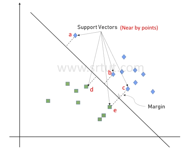
In Support Vector Machine (SVM), the margin refers to the distance between the decision boundary and the closest data points of each class. The goal of SVM is to find the hyperplane that separates the data points into different classes with the largest margin between them. The margin is important because it reflects the performance of the model. A larger margin implies that the model is less sensitive to small changes in the training data, and hence more likely to generalize well to new, unseen data.
Support Vectors
The nearby datapoints which are close to decision boundary, are called Support Vectors. In the given image points a,b,c and d, e are support vectors.
Decision Boundary

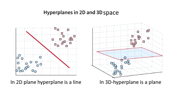
The decision boundary is the hyperplane that separates the data points of different classes. In a binary classification problem, the decision boundary is a line in 2D space, It is a plane in 3D space and a hyperplane in higher dimensional spaces. The decision boundary is learned during the training phase of the SVM model by maximizing the margin between the data points of different classes.
Types of SVMs
SVMs (Support Vector Machines) can be categorized into two types: linear and non-linear SVMs. The main difference between the two SVMs is, how they draw decision boundaries between classes.
Linear SVMs: Linear SVMs assume that the data can be separated by a straight line or hyperplane. The goal of the algorithm is to find the hyperplane that maximizes the margin (i.e., the distance between the hyperplane and the closest points of each class). The hyperplane can be described by a linear equation in the form of w⋅x + b = 0, where w is the weight vector and b is the bias term. The weight vector determines the direction of the hyperplane, while the bias term shifts the hyperplane in the desired direction.
Linear SVMs are used for binary classification problems where the data can be separated by a straight line or hyperplane. Let's consider an example of classifying whether a fruit is an apple or an orange based on its weight and diameter. We have a dataset of fruits with their corresponding weight and diameter, as shown below:
| Fruit | Weight(gms) | Diameter(cm) |
|---|---|---|
| Apple | 100 | 8 |
| Apple | 110 | 7 |
| Orange | 140 | 10 |
| Orange | 130 | 9 |
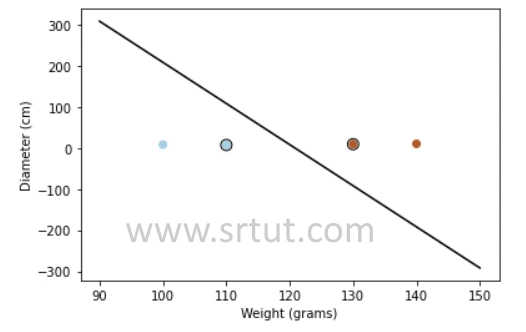
We can plot the data on a 2-dimensional space, with weight on the x-axis and diameter on the y-axis, as shown below:

We can see that the data is linearly separable, and we can draw a line (hyperplane) that separates the apples from the oranges. The line we choose should maximize the margin between the two classes. In this example, the line that maximizes the margin is shown as the solid line in the figure above.
Non-linear SVMs: Non-linear SVMs, on the other hand, are used when the data is not linearly separable. In such cases, SVMs use a technique called kernel trick to transform the data into a higher-dimensional space where it can be linearly separable. This means that SVMs find a decision boundary that is not linear in the original space but can be linear in a higher-dimensional space. Kernel functions such as polynomial, radial basis function (RBF), and sigmoid are commonly used to perform this transformation. Non-linear SVMs are more flexible in their ability to separate complex data, but they can also be more computationally expensive than linear SVMs.
Non-linear SVMs are used for binary classification problems where the data cannot be separated by a straight line or hyperplane in the original space. Consider an example where we want to classify whether a person has diabetes or not based on their glucose and insulin levels. We have a dataset of patients with their corresponding glucose and insulin levels, as shown below:
| Diabetes | Glucose Level | Insulin Level |
|---|---|---|
| No | 95 | 20 |
| No | 90 | 25 |
| Yes | 120 | 80 |
| Yes | 125 | 90 |
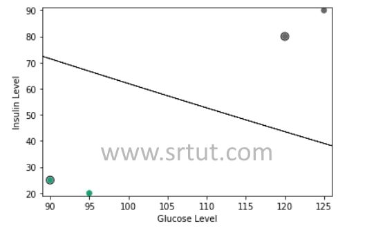
We can plot the data on a 2-dimensional space, with glucose level on the x-axis and insulin level on the y-axis, as shown below:

Steps of SVM Algorithm
- Data Preprocessing: First, we need to prepare our data for SVM. This includes removing any outliers or noise, handling missing values, and scaling the data to bring all features on the same scale.
- Selecting the Kernel: The next step is to choose the appropriate kernel function. The kernel function maps the input data into a higher-dimensional space where it can be linearly separated. There are different types of kernel functions, such as linear, polynomial, and radial basis function (RBF).
- Training the Model: In this step, we use the training dataset to create the SVM model. The SVM algorithm finds the hyperplane that maximizes the margin between the two classes. The margin is the distance between the hyperplane and the nearest data points of each class.
- Tuning the Hyperparameters: SVM has several hyperparameters that need to be optimized to improve the performance of the model. Some of the important hyperparameters include the regularization parameter (C), the kernel parameter (gamma), and the degree of the polynomial kernel.
- Testing the Model: Once the model is trained and optimized, we need to evaluate its performance on the test dataset. We can use various evaluation metrics such as accuracy, precision, recall, and F1-score to measure the performance of the model.
- Making Predictions: Finally, we can use the trained SVM model to make predictions on new data points. The SVM algorithm classifies the new data point based on its location with respect to the hyperplane. If it lies on one side of the hyperplane, it belongs to one class, and if it lies on the other side, it belongs to the other class.
Advantages of SVM
Support Vector Machines (SVMs) are a popular type of machine learning algorithm that can be used for classification, regression, and outlier detection. Some advantages of SVMs include:
- Effective in high-dimensional spaces: SVMs are effective in high-dimensional spaces, meaning they can handle datasets with many features or variables.
- Robust to outliers: SVMs are robust to outliers, meaning that they can still make accurate predictions even when there are a few data points that are different from the others.
- Memory efficient: SVMs use a subset of training points called support vectors, which means that they are memory efficient and can handle large datasets.
- Versatile: SVMs can be used for both linear and nonlinear data, making them a versatile algorithm that can handle a wide range of problems.
- Good for small datasets: SVMs are effective for small datasets, as they can generalize well with a limited number of training examples.
- Offers control over trade-off between overfitting and underfitting: SVMs offer a flexible trade-off between overfitting and underfitting, as they allow users to adjust the regularization parameter to control the complexity of the model.
Advertisement
Advertisement